Brian J. Knaus

Analysis of variance (ANOVA) attempts to address the question if two or more groups are on average different. We’ve previously addressed the linear model. In the linear model we ask whether the slope is different from zero and whether the y-intercept is different from zero. In ANOVA we have predetermined groups and consider the slope for each group to be zero while we ask teh question of whether these groups all have the same y-intercept.

Here we’ll simulate three groups of 10 samples. We’ll start by setting their averages (y-intercepts) to be the same.

myGroups <- as.factor(rep(1:3, each=10))
set.seed(99)
myTrait <- rnorm(n = length(myGroups), mean = 20, sd = 4)
boxplot(myTrait ~ myGroups)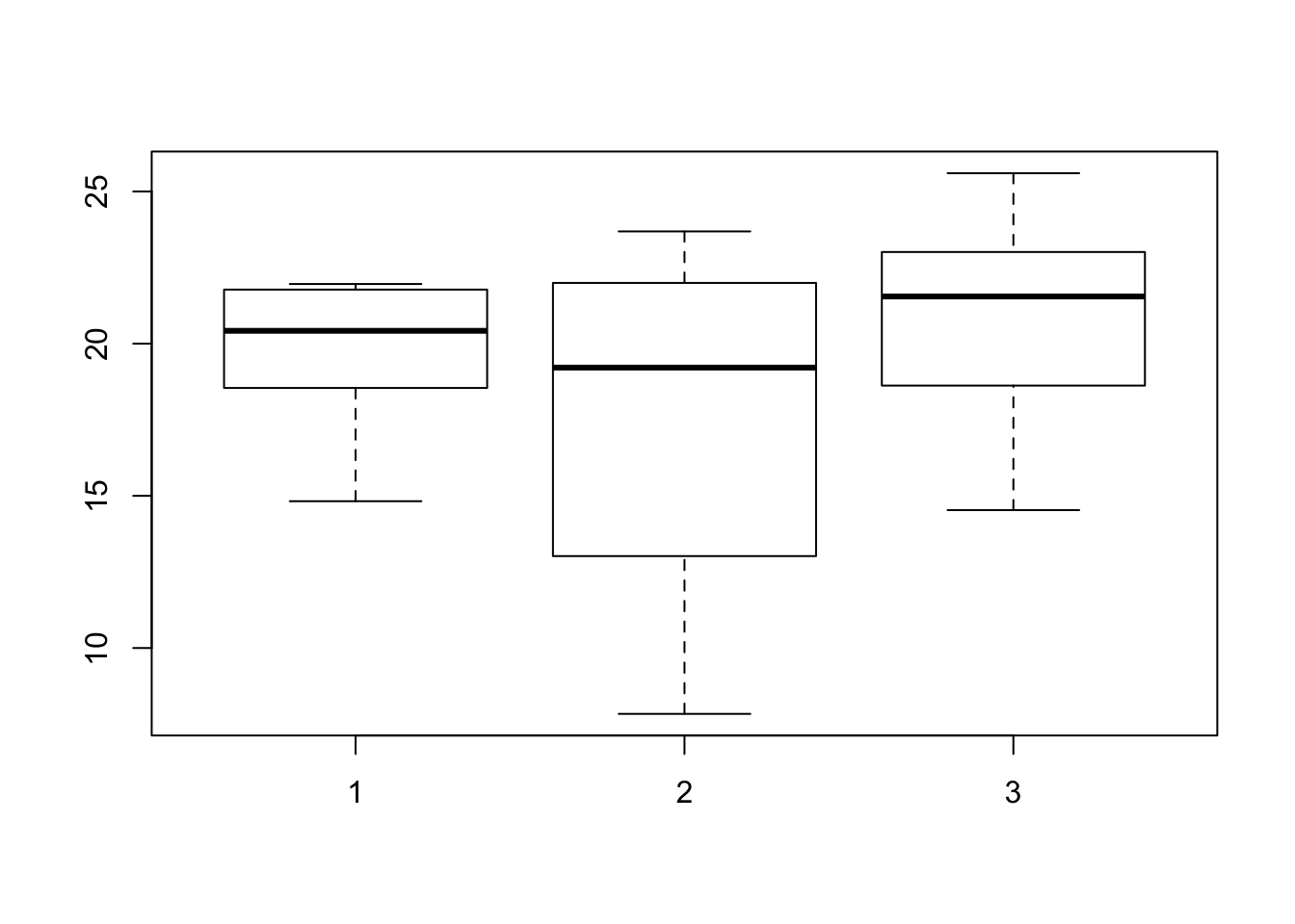

Box and whisker plots are a good way to visualize this data because it shows us the groupings and helps us determine if our data are normally distributed. Box and whisker plots also use the same syntax as our ANOVA functions. We can now test the data for different means. We have two functions to help us accomplish this so we’ll explore both of these.

lm1 <- aov(myTrait ~ myGroups)
summary(lm1)

##             Df Sum Sq Mean Sq F value Pr(>F)
## myGroups     2   56.9   28.43   1.775  0.189
## Residuals   27  432.4   16.01

lm2 <- lm(myTrait ~ myGroups)
summary(lm2)

## 
## Call:
## lm(formula = myTrait ~ myGroups)
## 
## Residuals:
##     Min      1Q  Median      3Q     Max 
## -9.7666 -2.0500  0.8654  2.3675  6.0833 
## 
## Coefficients:
##             Estimate Std. Error t value Pr(>|t|)    
## (Intercept)   19.581      1.265  15.473 6.05e-15 ***
## myGroups2     -1.978      1.790  -1.105    0.279    
## myGroups3      1.376      1.790   0.769    0.449    
## ---
## Signif. codes:  0 '***' 0.001 '**' 0.01 '*' 0.05 '.' 0.1 ' ' 1
## 
## Residual standard error: 4.002 on 27 degrees of freedom
## Multiple R-squared:  0.1162, Adjusted R-squared:  0.05074 
## F-statistic: 1.775 on 2 and 27 DF,  p-value: 0.1887

I prefer the second method because it prodces more details in the summary. Note that we can get similar information from each function’s result using accessor functions such as coefficients(lm1). So my preference here my be more due to habit than the amount of actual information provided. Note that this is the same function we used for our linear model. But because out independant variable (myGroups) is a factor the function knows that these are groups and performs an ANOVA. Feel free to explore what happens if we don’t use a factor.

The part of the output that we’re typically interested in is the coefficients table. The first row (Intercept) reports the mean value for the first group. We can validate this as follows.

mean(myTrait[myGroups == 1])

## [1] 19.58103

The p-value (Pr(>|t|)) reports this average to be significantly different from zero (i.e., it is less than 0.05). However, this is not our research question. So even though we’re typically interested in p-values that are less than 0.05 this is a situation where we are not interested in this p-value. The question we’re interested in is whether the subsequent groups differ from the first group. We see this on the subsequent rows of the table.

The second row (myGroups2) shows an estimate of -1.978. This is the difference between our intercept and the mean for the second group. We can validate this as follows.

sum(coefficients(lm2)[1:2])

## [1] 17.60286

mean(myTrait[myGroups == 2])

## [1] 17.60286

We can also view the box and whisker plot to see that the mean for the second group is lower than the first. While we do observe a difference, we see that the p-value is greater than 0.05 so we interpret this as a non-significant difference which is in agreement with how we simulated the data.

The third group is similar to the second in that it is also non-significantly different from the first group. We can validate these values as follows.

sum(coefficients(lm2)[c(1,3)])

## [1] 20.95691

mean(myTrait[myGroups == 3])

## [1] 20.95691

We’re typically interested in finding significant differences among our group. So let’s change our data so that there’s a difference.

set.seed(99)
myTrait[myGroups == 2] <- rnorm(n=sum(myGroups == 2), mean = 30, sd = 4)
boxplot(myTrait ~ myGroups)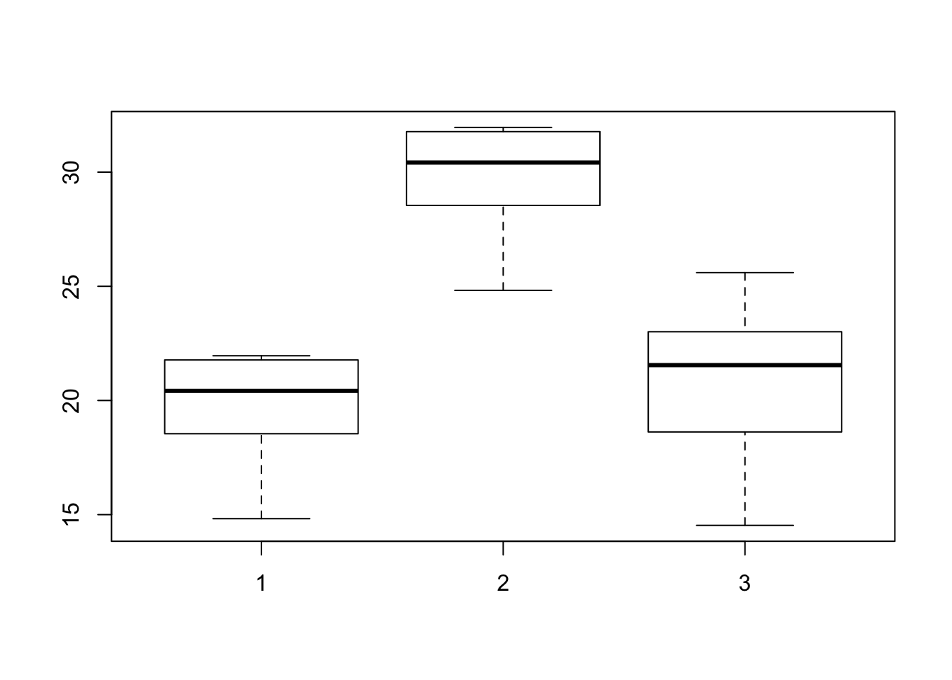

We now see a difference in group two’s mean. We can now test if it is a significant difference as we have above.

lm3 <- lm(myTrait ~ myGroups)
summary(lm3)

## 
## Call:
## lm(formula = myTrait ~ myGroups)
## 
## Residuals:
##    Min     1Q Median     3Q    Max 
## -6.427 -1.155  0.840  2.159  4.643 
## 
## Coefficients:
##             Estimate Std. Error t value Pr(>|t|)    
## (Intercept)  19.5810     0.8742  22.399  < 2e-16 ***
## myGroups2    10.0000     1.2363   8.089 1.09e-08 ***
## myGroups3     1.3759     1.2363   1.113    0.276    
## ---
## Signif. codes:  0 '***' 0.001 '**' 0.01 '*' 0.05 '.' 0.1 ' ' 1
## 
## Residual standard error: 2.764 on 27 degrees of freedom
## Multiple R-squared:  0.7401, Adjusted R-squared:  0.7209 
## F-statistic: 38.44 on 2 and 27 DF,  p-value: 1.258e-08

We see that the estimate for the first group (Intercept) and third group (myGroups3) are the same as the previous table. This is expected because we have not changed these. The estimate for the second group has changed and is now estimated to be 10. This actually matched our simulation quite well. We can validate our results as follows.

sum(coefficients(lm3)[1:2])

## [1] 29.58103

mean(myTrait[myGroups == 2])

## [1] 29.58103

We’ve used normal distributions to simulate our data. This is because standard ANOVA makes the assumption that the data is normally distributed. See the post on the linear model if you need a reminder of why this is. But how do we know if we’ve violated this assumption? One way is to see if the residuals are normally distributed. The residuals are how different each sample is from its group mean. We can visualize this with a histogram and a Q-Q plot.

par(mfrow=c(1,2))
hist(residuals(lm3))
qqnorm(residuals(lm3))
qqline(residuals(lm3))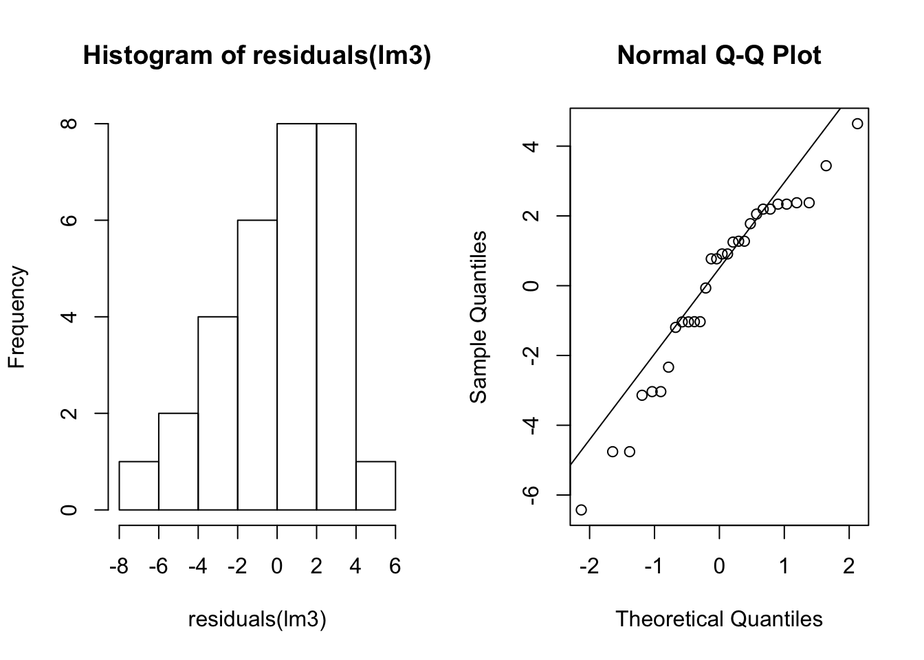

par(mfrow=c(1,1))

Note that the data do not appear perfectly normally distributed even though we sampled them from normal distributions. We also may want a test for normality. Here we us the Shapiro-Wilks test.

shapiro.test(residuals(lm3))

## 
##  Shapiro-Wilk normality test
## 
## data:  residuals(lm3)
## W = 0.94009, p-value = 0.09146

This tests the null hypothesis that the data are normally distributed. If the p-value were significant it would indicate a deviation from normality. Again note that even though we sampled the data from normal distributions our p-value is 0.09 which is non-significant but actually a bit surprisingly small.