Brian J. Knaus

The linear model is the foundation for much of statistical hypothesis testing. As such, it should be a foundational part of any scientist’s education and career. Unfortunately, it is frequently misunderstood. Here I attempt to explain the linear model with the hope of bringing clarity to the topic.

The linear model is based on the equation for a line, something we all learned in grade school geometry.

y = mx + b

Here y is a vector of our response or dependent variables. It is determined by the right hand side of the equation. On the right hand side of the equation we have m, which is our slope, x, our vector of independent variables, and b the y-intercept where x equals zero. We can display this in R as follows.

x <- 1:20
y <- 0.5 * x + 1
plot(x, y)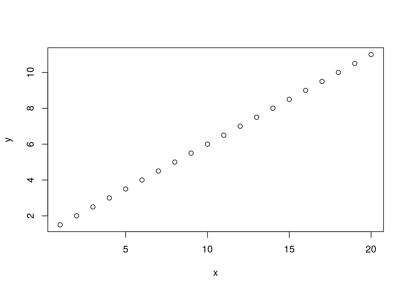  

If you’re familiar with biological data you probably know that this plot is unrealistic. Biological data rarely follows such a straight line. In order to accomodate deviations from our ‘perfect’ model we include an error term. Here we’ll add some normally distributed ‘error’ to our model. Mathematically we can represent this as follows.

y = mx + b + \epsilon

This can be represented in R as follows.

set.seed(9)
y <- 0.5 * x + 2 + rnorm(n=length(x))
plot(x, y)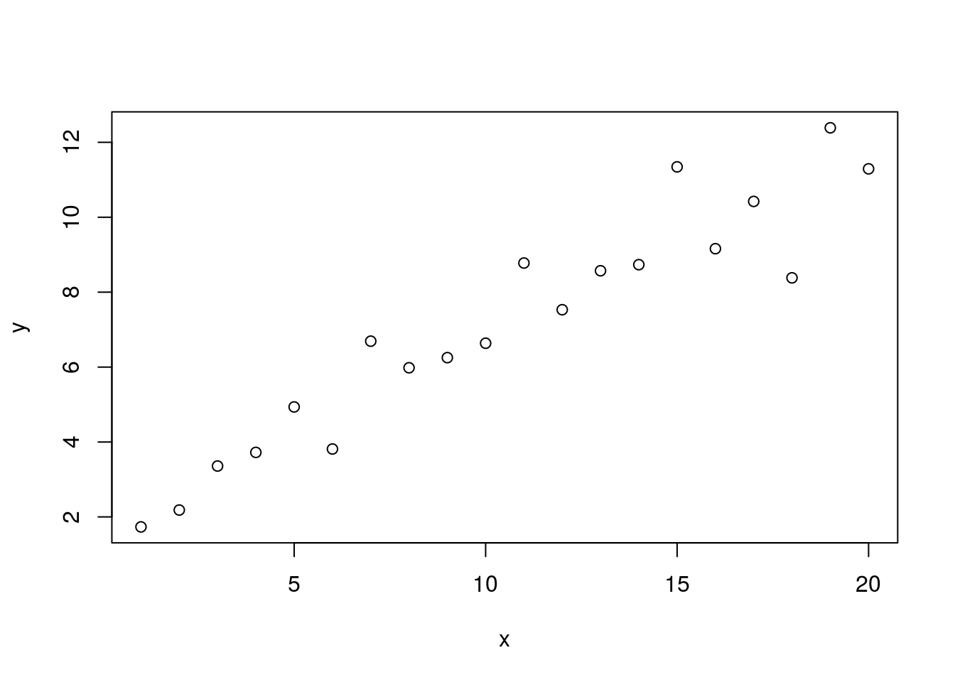

We no longer have a nice neat line. But we can see that the scatter of dots still appears to have an upward angle. We can model this with the function lm.

lm1 <- lm(y ~ x)
summary(lm1)

## 
## Call:
## lm(formula = y ~ x)
## 
## Residuals:
##     Min      1Q  Median      3Q     Max 
## -2.4636 -0.5682 -0.1028  0.3166  1.9994 
## 
## Coefficients:
##             Estimate Std. Error t value Pr(>|t|)    
## (Intercept)  1.84546    0.46805   3.943 0.000954 ***
## x            0.50003    0.03907  12.797 1.78e-10 ***
## ---
## Signif. codes:  0 '***' 0.001 '**' 0.01 '*' 0.05 '.' 0.1 ' ' 1
## 
## Residual standard error: 1.008 on 18 degrees of freedom
## Multiple R-squared:  0.901,  Adjusted R-squared:  0.8955 
## F-statistic: 163.8 on 1 and 18 DF,  p-value: 1.779e-10

From the Coefficients table we see tha intercept to be estimated to be 1.8 and that it’s p-value is less than 0.05 indicating that it is significantly different from zero. Compare this estimate (1.8) to it’s actual value above (2) and I think you will see that they are very similar. We can also see that the estimate of our slope (0.5) is very close to it’s actual value (0.5) and the p-value is significant (below 0.05).

Note that we are testing two hypotheses here. We are testing whether the intercept is different from zero and we’re testing whether the slope is different from zero. We can validate this by simulating new data where these values are closer to zero. First we’ll change the y-intercept.

set.seed(9)
y <- 0.5 * x + 0.2 + rnorm(n=length(x))
plot(x, y)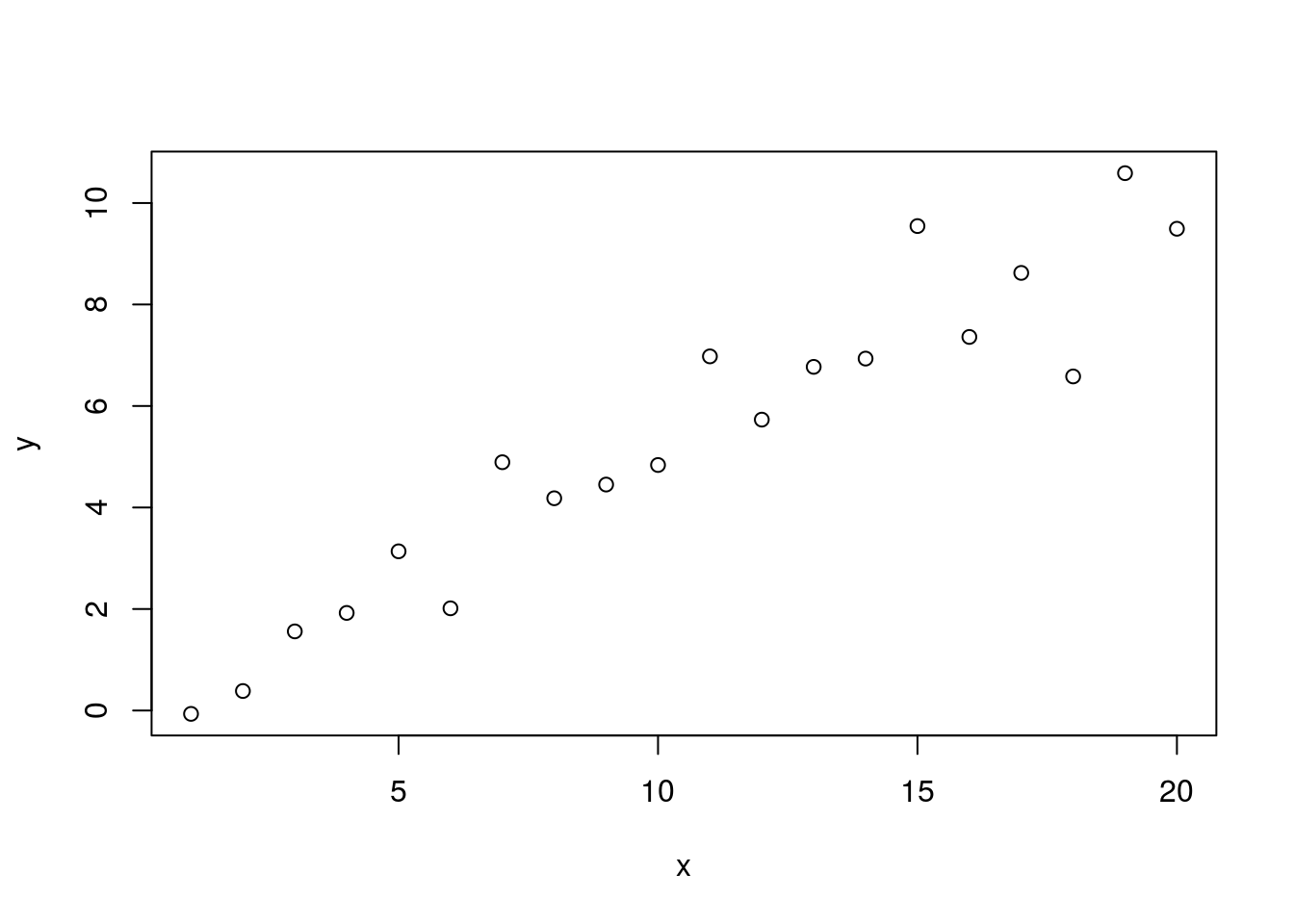

lm2 <- lm(y ~ x)
summary(lm2)

## 
## Call:
## lm(formula = y ~ x)
## 
## Residuals:
##     Min      1Q  Median      3Q     Max 
## -2.4636 -0.5682 -0.1028  0.3166  1.9994 
## 
## Coefficients:
##             Estimate Std. Error t value Pr(>|t|)    
## (Intercept)  0.04546    0.46805   0.097    0.924    
## x            0.50003    0.03907  12.797 1.78e-10 ***
## ---
## Signif. codes:  0 '***' 0.001 '**' 0.01 '*' 0.05 '.' 0.1 ' ' 1
## 
## Residual standard error: 1.008 on 18 degrees of freedom
## Multiple R-squared:  0.901,  Adjusted R-squared:  0.8955 
## F-statistic: 163.8 on 1 and 18 DF,  p-value: 1.779e-10

Here we’ve changed the y-intercept from 2 to 0.2. Our linear model now estimates the intercept to be -0.386 but because the p-value is greater than 0.05 we conclude that it is not significantly different from zero. This validates that our coefficient for the intercept tests whether it is different from zero. We can perform a similar validation for the slope.

set.seed(9)
y <- 0.02 * x + 2 + rnorm(n=length(x))
plot(x, y)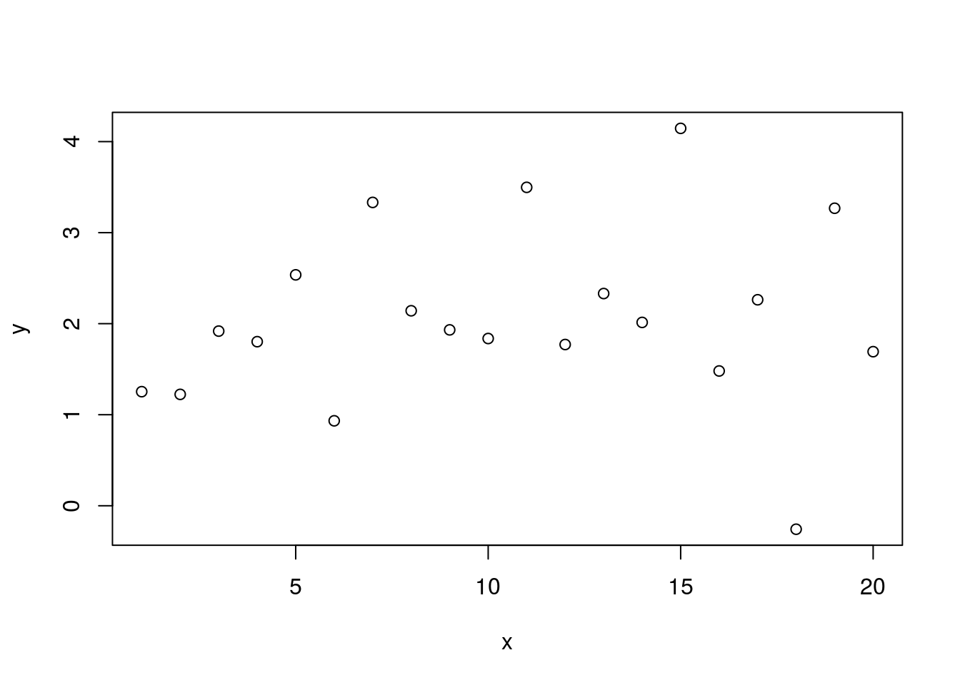

lm3 <- lm(y ~ x)
summary(lm3)

## 
## Call:
## lm(formula = y ~ x)
## 
## Residuals:
##     Min      1Q  Median      3Q     Max 
## -2.4636 -0.5682 -0.1028  0.3166  1.9994 
## 
## Coefficients:
##             Estimate Std. Error t value Pr(>|t|)    
## (Intercept)  1.84546    0.46805   3.943 0.000954 ***
## x            0.02003    0.03907   0.513 0.614514    
## ---
## Signif. codes:  0 '***' 0.001 '**' 0.01 '*' 0.05 '.' 0.1 ' ' 1
## 
## Residual standard error: 1.008 on 18 degrees of freedom
## Multiple R-squared:  0.01438,    Adjusted R-squared:  -0.04037 
## F-statistic: 0.2627 on 1 and 18 DF,  p-value: 0.6145

Here we’ve returned our value for the y-intercept to 2 and it returns to being statistically significantly different from zero. But our slope is now set to 0.02. It’s actually well estimated by the model at 0.02, but this is not significantly different from zero based on the large p-value.

The linear model is a fundamental part of statistical hypothesis testing. Here we’ve shown that the linear model can be used to test if the y-intercept of a relationship of data are significantly different from zero and if the slope among data are significantly different from zero. And we’ve shown that these hypothesees can be tested independantly of one another. The linear model can be seen as an effective tool to test for relationships among data.