Edgar Anderson’s Irises
This data set consistst of four continuous characters collected for three species of Iris. The data were assembled by Anderson (1935) and famously analysed by Fisher (1936). It is a nice dataset because it is reasonably small. This makes it easy to visualize. It also makes it a good daata set when trying to learn new analyses, particularly when the data set intende to be analysed is much larger. It is also a part of R so most intallations should have it. It can be loaded as follows.
data("iris")More information can be found using ?iris.
We can visualize this data using histograms.
library(ggplot2)
library(reshape2)
iris2 <- melt(iris)
## Using Species as id variablesp <- ggplot(iris2, aes(x=value, fill = Species))
p <- p + geom_histogram(binwidth = 0.2, alpha=.5)
p <- p + facet_grid(. ~ variable, scales = "free")
p <- p + scale_fill_manual(values=c("#66c2a5", "#fc8d62", "#8da0cb"))
p <- p + xlab("Length")
p <- p + ylab("Count")
p <- p + theme_bw()p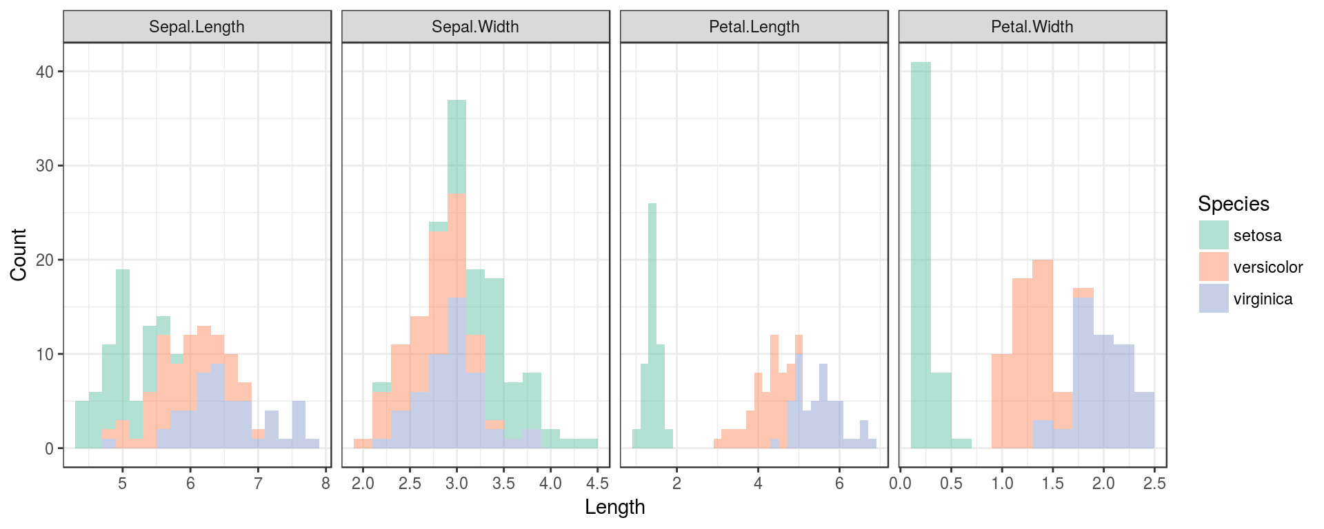
An alternative perspective would be violin plots.
p <- ggplot(iris2, aes(x=Species, y=value, fill = Species))
p <- p + geom_violin()
p <- p + scale_fill_manual(values=c("#66c2a5", "#fc8d62", "#8da0cb"))
p <- p + facet_grid(. ~ variable)
p <- p + xlab("")
p <- p + ylab("Length")
p <- p + theme_bw()
p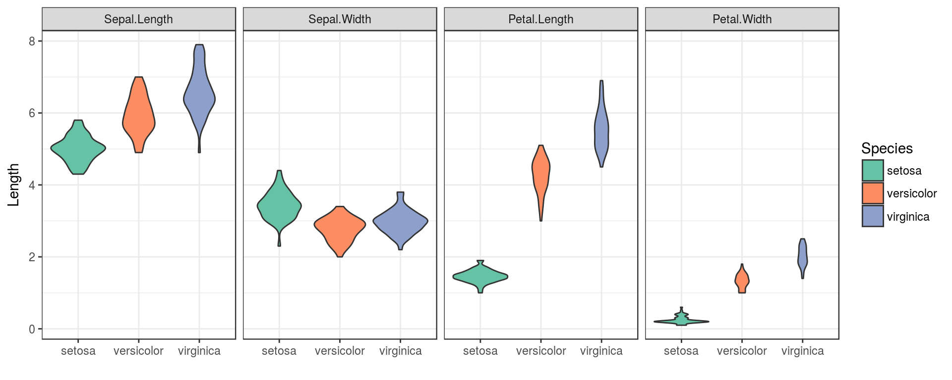
References
Anderson, Edgar. 1935. “The Irises of the Gaspe Peninsula.” Bulletin of the American Iris Society 59: 2–5.
Fisher, Ronald A. 1936. “The Use of Multiple Measurements in Taxonomic Problems.” Annals of Eugenics 7 (2). Wiley Online Library: 179–88.
Copyright © Brian J. Knaus. All rights reserved.