vcfR documentation
byBrian J. Knaus and Niklaus J. Grünwald
Filtering data
The output of variant calling pipelines result in files containing called variants. Many of these pipelines recommend further filtering of this data to ensure that only high quality variants are included in downstream analyses. In this vignette I discuss strategies to focus on the high quality fraction of these variants.
Data input
As in other vignettes, we begin by loading the example data. Here we’ll use this data to create a chromR object directly after inputting the data.
library(vcfR)

vcf_file <- system.file("extdata", "pinf_sc50.vcf.gz", package = "pinfsc50")
dna_file <- system.file("extdata", "pinf_sc50.fasta", package = "pinfsc50")
gff_file <- system.file("extdata", "pinf_sc50.gff", package = "pinfsc50")

vcf <- read.vcfR(vcf_file, verbose = FALSE)
dna <- ape::read.dna(dna_file, format = "fasta")
gff <- read.table(gff_file, sep="\t", quote="")

chrom <- create.chromR(name="Supercontig", vcf=vcf, seq=dna, ann=gff, verbose=FALSE)
chrom <- proc.chromR(chrom, verbose = TRUE)
## Nucleotide regions complete.## elapsed time: 0.328## N regions complete.## elapsed time: 0.369## Population summary complete.## elapsed time: 0.315## window_init complete.## elapsed time: 0## windowize_fasta complete.## elapsed time: 0.118## windowize_annotations complete.## elapsed time: 0.02## windowize_variants complete.## elapsed time: 0.003Using a mask
Instead of removing variants, vcfR implements a mask. This allows changes to be easily undone and it preserves the geometry of the data matrix. Preserving the geometry of the matrix also allows for multiple manipulations to be made easily. When we’ve settled on a set of manipulations which we like we can then use this mask to subset the data.
The function masker() censors variants (i.e., sets the mask) based on several thresholds. A number of summaries regarding variant quality are reported in VCF files. These summaries may differ in content depending on what software was used to create them, as well as what options may have been used. For example, a quality metric may range from 0 to 20 or 0 to 100 depending on choices made by the developer (i.e., are they raw probabilities or phred converted, etc.). Because of this, the default values for masker() are not likely to be very useful. The user will need to explore their data to identify useful thresholds. We can use the head() function to see what sort of information is contained in our data.
head(chrom)## ***** Class chromR, method head *****
## Name: Supercontig
## Length: 1,042,442
##
## ***** Sample names (chromR) *****
## [1] "BL2009P4_us23" "DDR7602" "IN2009T1_us22" "LBUS5"
## [5] "NL07434" "P10127"
## [1] "..."
## [1] "P17777us22" "P6096" "P7722" "RS2009P1_us8" "blue13"
## [6] "t30-4"
##
## ***** VCF fixed data (chromR) *****
## CHROM POS ID REF ALT QUAL FILTER
## [1,] "Supercontig_1.50" "41" NA "AT" "A" "4784.43" NA
## [2,] "Supercontig_1.50" "136" NA "A" "C" "550.27" NA
## [3,] "Supercontig_1.50" "254" NA "T" "G" "774.44" NA
## [4,] "Supercontig_1.50" "275" NA "A" "G" "714.53" NA
## [5,] "Supercontig_1.50" "386" NA "T" "G" "876.55" NA
## [6,] "Supercontig_1.50" "462" NA "T" "G" "1301.07" NA
## [1] "..."
## CHROM POS ID REF ALT QUAL FILTER
## [22026,] "Supercontig_1.50" "1042176" NA "T" "A" "162.59" NA
## [22027,] "Supercontig_1.50" "1042196" NA "G" "A" "180.86" NA
## [22028,] "Supercontig_1.50" "1042198" NA "T" "G" "60.27" NA
## [22029,] "Supercontig_1.50" "1042303" NA "C" "G" "804.15" NA
## [22030,] "Supercontig_1.50" "1042396" NA "GA" "G" "1578.82" NA
## [22031,] "Supercontig_1.50" "1042398" NA "A" "C" "1587.87" NA
##
## INFO column has been suppressed, first INFO record:
## [1] "AC=32" "AF=1.00"
## [3] "AN=32" "DP=174"
## [5] "FS=0.000" "InbreedingCoeff=-0.0224"
## [7] "MLEAC=32" "MLEAF=1.00"
## [9] "MQ=51.30" "MQ0=0"
## [11] "QD=27.50" "SOR=4.103"
##
## ***** VCF genotype data (chromR) *****
## ***** First 6 columns *********
## FORMAT BL2009P4_us23 DDR7602
## [1,] "GT:AD:DP:GQ:PL" "1|1:0,7:7:21:283,21,0" "1|1:0,6:6:18:243,18,0"
## [2,] "GT:AD:DP:GQ:PL" "0|0:12,0:12:36:0,36,427" "0|0:20,0:20:60:0,60,819"
## [3,] "GT:AD:DP:GQ:PL" "0|0:27,0:27:81:0,81,1117" "0|0:26,0:26:78:0,78,1077"
## [4,] "GT:AD:DP:GQ:PL" "0|0:29,0:29:87:0,87,1243" "0|0:27,0:27:81:0,81,1158"
## [5,] "GT:AD:DP:GQ:PL" "0|0:26,0:26:78:0,78,1034" "0|0:30,0:30:90:0,90,1242"
## [6,] "GT:AD:DP:GQ:PL" "0|0:23,0:23:69:0,69,958" "0|0:36,0:36:99:0,108,1556"
## IN2009T1_us22 LBUS5
## [1,] "1|1:0,8:8:24:324,24,0" "1|1:0,6:6:18:243,18,0"
## [2,] "0|0:16,0:16:48:0,48,650" "0|0:20,0:20:60:0,60,819"
## [3,] "0|0:23,0:23:69:0,69,946" "0|0:26,0:26:78:0,78,1077"
## [4,] "0|0:32,0:32:96:0,96,1299" "0|0:27,0:27:81:0,81,1158"
## [5,] "0|0:41,0:41:99:0,122,1613" "0|0:30,0:30:90:0,90,1242"
## [6,] "0|0:35,0:35:99:0,105,1467" "0|0:36,0:36:99:0,108,1556"
## NL07434
## [1,] "1|1:0,12:12:36:486,36,0"
## [2,] "0|0:28,0:28:84:0,84,948"
## [3,] "0|1:19,20:39:99:565,0,559"
## [4,] "0|1:19,19:38:99:523,0,535"
## [5,] "0|1:22,22:44:99:593,0,651"
## [6,] "0|1:29,25:54:99:723,0,876"
##
## ***** Var info (chromR) *****
## ***** First 6 columns *****
## CHROM POS MQ DP mask n
## 1 Supercontig_1.50 41 51.30 174 TRUE 16
## 2 Supercontig_1.50 136 52.83 390 TRUE 17
## 3 Supercontig_1.50 254 56.79 514 TRUE 17
## 4 Supercontig_1.50 275 57.07 514 TRUE 17
## 5 Supercontig_1.50 386 57.40 509 TRUE 16
## 6 Supercontig_1.50 462 58.89 508 TRUE 17
##
## ***** VCF mask (chromR) *****
## Percent unmasked: 100
##
## ***** End head (chromR) *****The masker() function uses QUAL, sequence depth and mapping quality to try to filter out low quality variants. The parameter QUAL is a part of the VCF file definition. Because of this, it is not documented in the meta region. This parameter should always be present. However, it may be set to missing (‘.’ in the file, NA as read in by vcfR) or populated with a constant, both of which render this metric as unuseful. The parameters DP and MQ are in the INFO column an are not part of the VCF definition. The parameter DP is not a required field, so it is defined in the meta region.
We can remind ourselves how these parameters are defined by querying the meta region.
strwrap(grep("ID=MQ,", chrom@vcf@meta, value = T))## [1] "##INFO=<ID=MQ,Number=1,Type=Float,Description=\"RMS Mapping Quality\">"strwrap(grep("ID=DP,", chrom@vcf@meta, value = T))## [1] "##FORMAT=<ID=DP,Number=1,Type=Integer,Description=\"Approximate read"
## [2] "depth (reads with MQ=255 or with bad mates are filtered)\">"
## [3] "##INFO=<ID=DP,Number=1,Type=Integer,Description=\"Approximate read"
## [4] "depth; some reads may have been filtered\">"We see that ‘DP’ has different definitions in the INFO column than in the genotype region. The discrepancy appears to be due to some variants which have a high number of raw reads but only a fraction of these have been determined to be of high quality. Because masker() uses the DP column in the var.info slot to judge depth, we’ll change it to include only the high quality depth.
We can now use the plot function to visualize this data.
plot(chrom)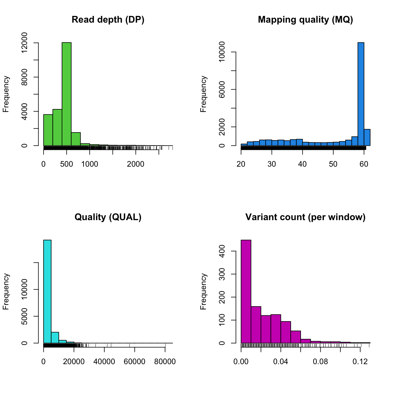
Our summary of DP appears continuous. However, we do have variants which appear to have unusually low coverage which we may try to filter out. We also see that DP is very long tailed in that it has a number of variants with exceptionally high coverage. These typically come from repetetive regions that have reads which map to multiple locations in the genome. Mapping quality is largely of one value (60). But there are some lower values which we may want to remove. Quality is notable in that it is fairly clinal and may not be useful for filtering.
We can also use the chromoqc function to see how the data are distributed along the chromosome.
chromoqc(chrom, dp.alpha = 22)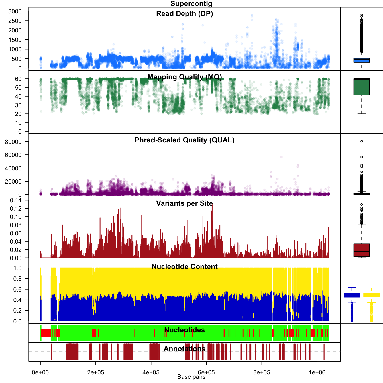
Now that we have our first peek at the data, we can try to parameterize the masker function to isolate variants we feel to be of high quality.
chrom <- masker(chrom, min_QUAL=0, min_DP=350, max_DP=650, min_MQ=59.5, max_MQ=60.5)
chrom <- proc.chromR(chrom, verbose = FALSE)
plot(chrom)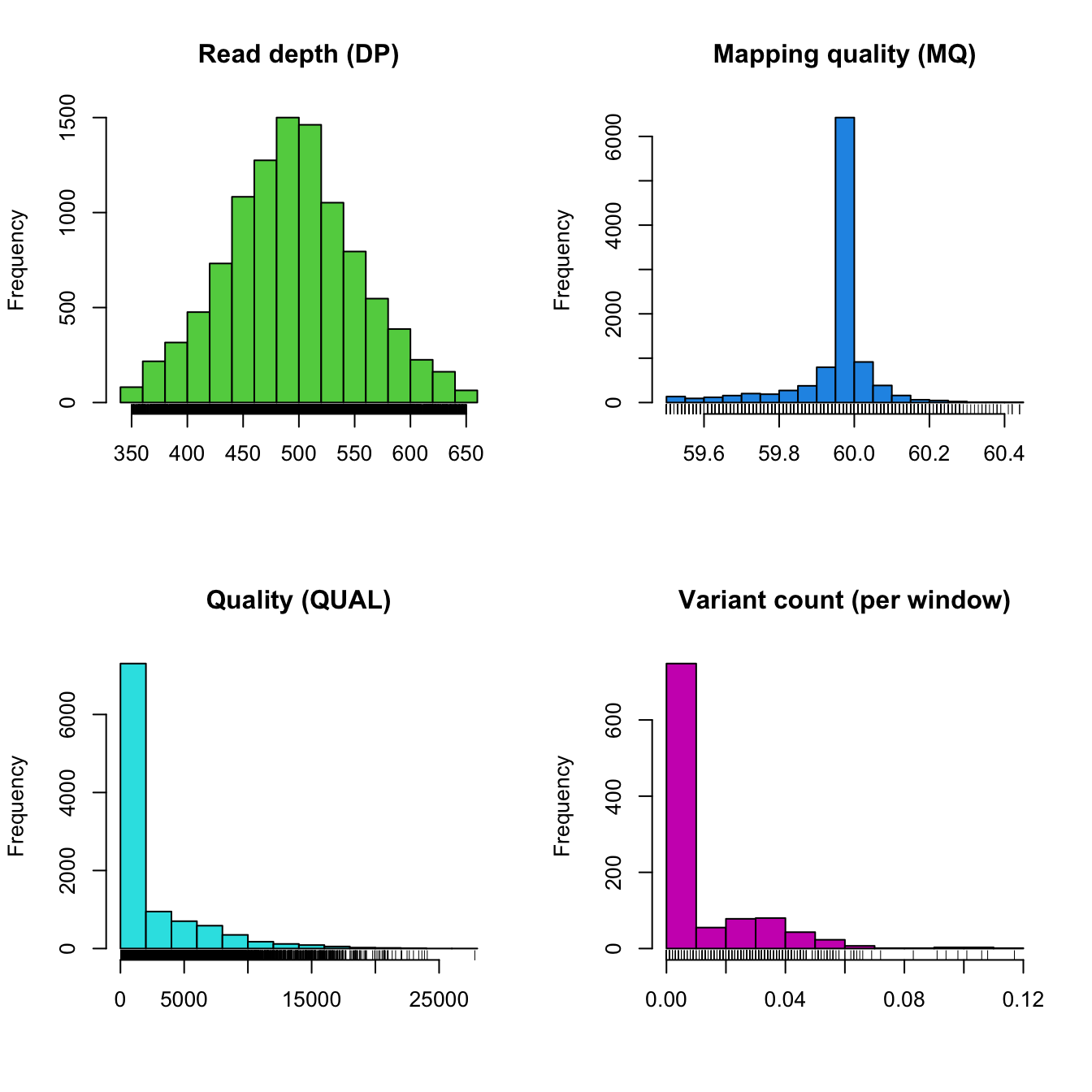
Note that we need to run proc.chrom() again. This will update the variant count per window.
The distribution of our read depths has now become narrower and excludes low coverage variants, it is also fairly symmetric. The distribution of mapping quality has also become more narrow. Note that while in this example we were able to rapidly pick relatively good thresholds. This was the result of some trial and error. The user should expect this process to take a few attempts.
We can use chromoqc() to see how applying this mask affects our data.
chromoqc(chrom, dp.alpha = 22)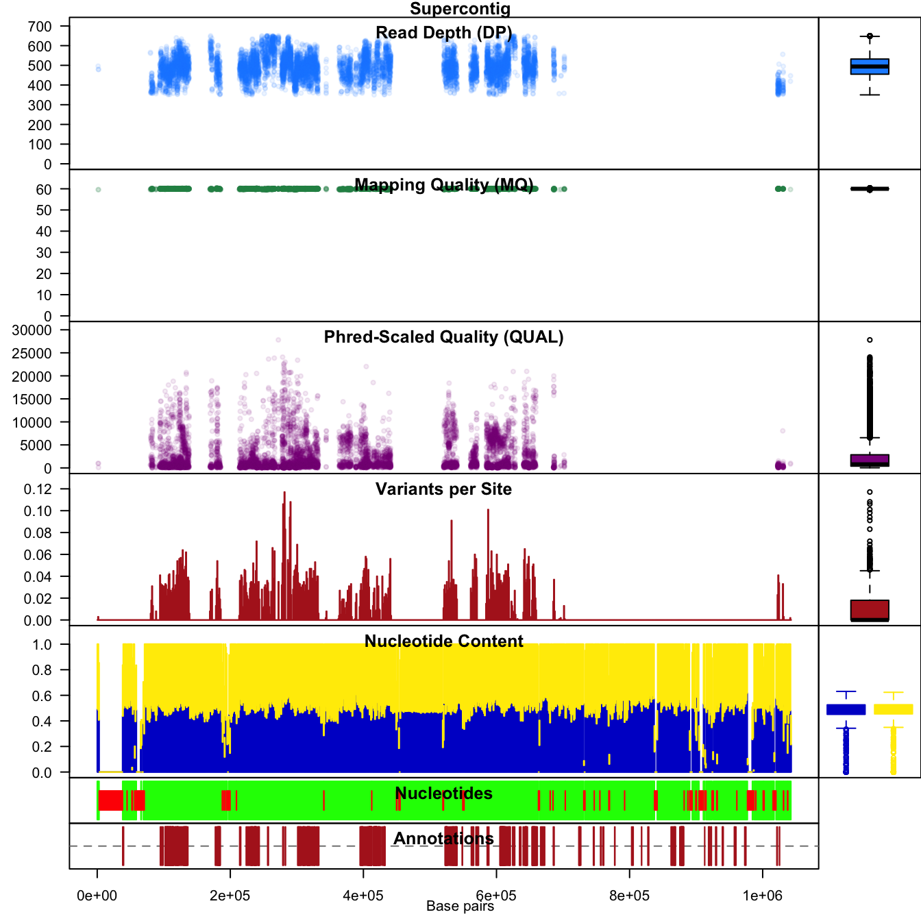
The chromo plot shows us that the variants of low quality populated the 3’ end of the supercontig. Filtering has removed all of the variants from this region. Use of stringent filtering may be used to build a conservative set of variants. This conservative set may be used for analysis or it may be used as a training set for subsequent rounds of variant discovery.
Output
Once satisfactory filtering has been completed you’ll want to save this high quality set of variants. This can be done by writing these variants to a new VCF file with the function write.vcf().
write.vcf(chrom, file="good_variants.vcf.gz", mask=TRUE)Copyright © 2017, 2018 Brian J. Knaus. All rights reserved.
USDA Agricultural Research Service, Horticultural Crops Research Lab.